Oscillatory–Rotational Interpretation of Atomic Orbitals
Bi-Resonant Roton
We try to continue the “Rotonal approach” of the Atom Model into rotations and resonances by different radii and spatial directions. So we have a central orbital of 2 electrons usually called 1s orbital with a normalized radius of 1. Second we have a 2 electron orbital called 2s and a relative radius of 4. These orbitals are sometimes shown as spherical objects, but this might only be the case because measurements can not distinguish directions. So let’s say they are circles and the 1s and 2s Rotons are Co-Axial.
Now having 2 radii, we can have further oscillation variants by letting electrons rotate (or rather oscillate) in X-Direction with a radius of 4 and in Y-Direction with a radius of 1 using the appropriate oscillation frequency of that direction. The frequency in each direction has to be adjusted such, that the curve closes onto itself after some multiples of $2*pi$.
Visualizations
2D Resonance Projection
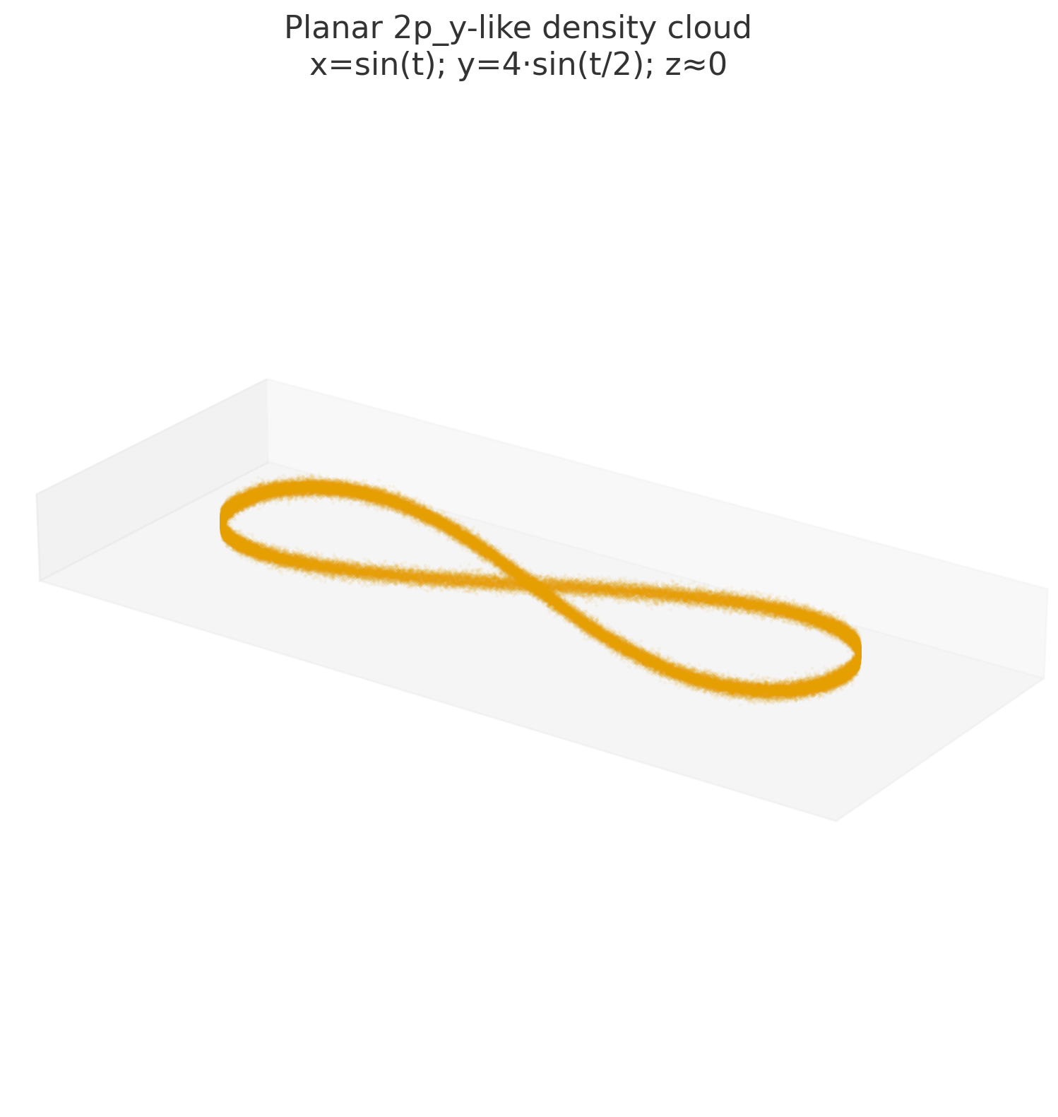
Projecting the resulting Figure onto a plane results in the following orbital:
- Calculation of a 4-1-0 resonance orbital 2p_y planar density cloud

3D Resonance Projection (1 Electron)
There are different methods for a spatial calculation of an electron orbital fulfilling this restrictions.
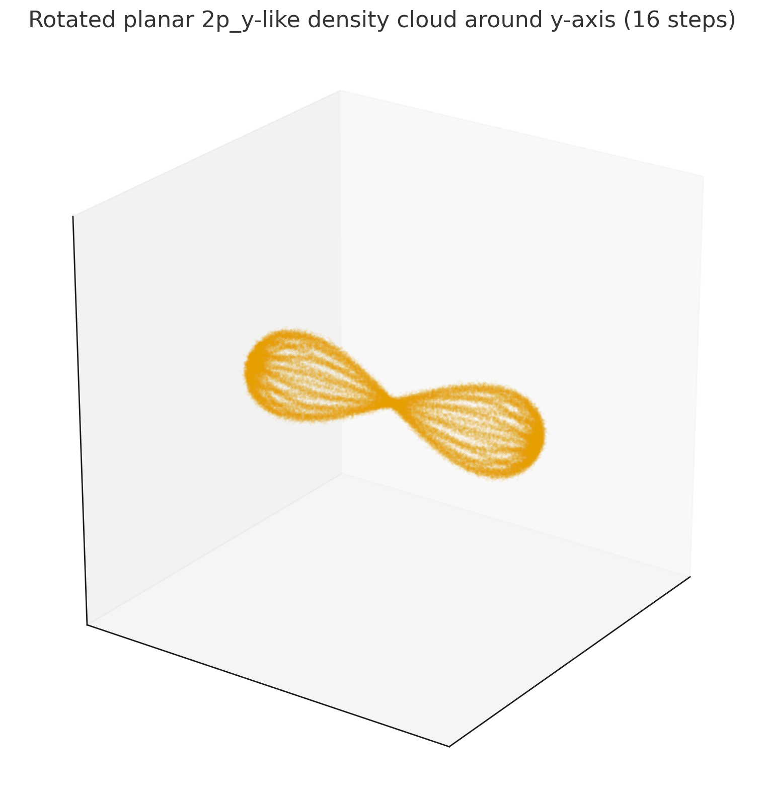
If we start with a planar rotation and adding tilts in x and y direction we can even have a single electron on the outer shell show these projections:

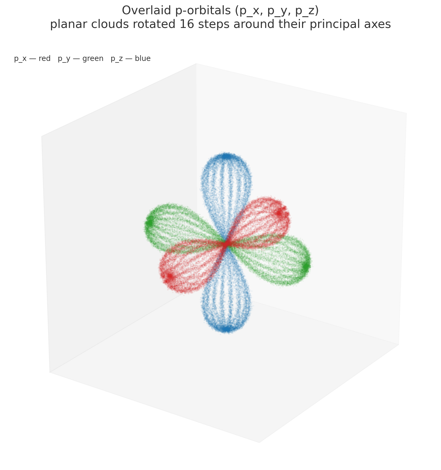
So the complex orbitals of the standard atom model can simply be described as a combinatorics composition of rotations with different resonant directions and amplitudes.
Standard Visualization of orbitals
If we “artificially” rotate these orbitals around their axis, we come up with the “well known” structure of the 2p orbitals with the second shell.

This though comes with some caveats. With this visualization, the electrons are NOT actually rotating within the n=2 shell anymore. And everybody asks, well why does the electron potentially come so close to the nucleus? Well we know it’s just a probability function, but where does the electron wave pass so that a single electron can build this 2 lope structure? Let’s explain it differently.
These “probability clouds” unfortunately are still projections of a sum of possible individual electron paths. And even worse, they are projections in different directions combined into one 3D image. So we see a suggested state of an atom, with places for electrons which they actually never take in the shown constellations. But lets first start with the basics, before moaning about the standard atom model.
Olavian atom model
This model reformulates classical electron orbitals as effective paths of a 3D oscillation systems, each defined by resonance amplitudes along the three spatial axes (x, y, z). For the first step (2 resonance amplitudes) the electron path can maintain a rotation within the 2p plain where the second resonance is fulfilled by a precession (tilt) of the rotation axis.
Each orbital is represented by a numeric triplet:
$$ (A_x, A_y, A_z) $$
where each component corresponds to a radial resonance level (1, 4, 9, 16 …),
reflecting the effective oscillation amplitude or energy radius on that axis ($1^2, 2^2, 3^3, …$).
The second triple describes the relative frequency of the oscillations (_222=2Pi/t in x, precession of 2pi/t in y an z).
Note: The “real” oscillation-frequency along the precession axis, would effectively be factor two. This is 244 for the frequency in yxz. But I’ll keep the labeling of the used simulation scripts.
| p2x_410_222 | p2z_411_222 | p3x_940_333 | s3_900_333 |
|---|---|---|---|
 |
|
 |
 |
Electron pairing
As known from experiments, the orbitals show their corresponding 2 lope scattering even in cases, where they are only filled with one electron. Furthermore, the p orbitals are first filled by one electron in each direction (x,y,z). How can this be explained with the precession approach?
The simplest Roton-projection with two frequencies shows, that the resulting curve in space is not point-symmetric to the atom center. So a energetically optimal quad-roton entangled system (Electron-Proton-Proton-Electron) can not be built with 2 electrons being on the same resonance rotation path. So this “orbital” is actually a single-Orbital. Luckily we can place a second electron on the other side with a mirrored path to reach this electron pairing. Each electron has its own “path” but the orbital-projections still align. The following illustration makes this clear very intuitively.
 [Image: Two electrons (green/blue) in a 2p shell with different paths but identical projections. Opposite to each other via the nucleus during the whole path.]
Torsodial paths
This is the place where we again have to extend the original intended single Rotations and the resulting Roton. The LEDO-Field allows more types of resonances than pure 2D planar rotations. A Roton though is the “simplest” type of self-sustained entity. We introduce a new name for a compound-rotation and an entity which follows such a spatially combined rotation path.
Discrepancy of Olavian Resonance Paths to the standard Orbital
Why does the Roton view show a closed electron path that differs from the standard symmetric orbital images? And why do we nevertheless see these standard orbital lobes in the planar projections of these 3D curves?
In short: The Schrödinger equations basically provide 2D and axially symmetrical solutions in 3D space for the wave-functions for single electrons. A little longer: If we measure statistically we get a distribution cloud of a excited, wobbling and rotating closed electron path.
Calculation of compound Wavefunctions extending single quantum eigenstates
For the more mathematically interested reader please find some considerations and calculation attempts here: Schrödinger equation for Olavion p2 Orbitals
Influence of Measurement on Atomic Orbital Imaging
Does the interpretation of the Olavian A Model match to what the experiments show?
(1) Standard Physics View
Orbital “shapes” are reconstructed from measurements made under controlled fields (electric, magnetic, laser, or scattering). These fields define an axis, lift degeneracy, and allow the probability density $|\psi(\mathbf r)|^2$ to be inferred from many ionization or scattering events.
The resulting lobes are field-aligned, ensemble-averaged densities, not direct pictures of free atoms.
(2) Key Objections and resulting Influence Concerns
- We never observe a supposedly “neutral” atom; the field needed for alignment already imposes directionality.
- Measurements from various sides may sample different states, not different projections of one fixed configuration.
- The measurement as such has influence on the observed atom and alters its state.
- Rotational motion during acquisition could artificially create symmetry.
- The reconstructed orbital may therefore describe a measurement-induced configuration, not an intrinsic 3D form.
(3) Resulting Influence Concerns
- A. Field Induced alignment: the field fixes one spatial direction, possibly giving the illusion of a full 3D structure.
- B. Cumulative conditioning: repeated probing continually prepares the system in the very state being measured.
- C. Triggered wobbling: the initial measurement interaction excites oscillations; we might record only a transient wobbling state.
- D. Measurement Induced alignment: the measurement itself (e.g. scattering direction) fixes a second spatial direction, giving the illusion of seeing the full 3D structure.
- E. Rotation around the field axis: time-averaging over such motion yields a falsely symmetric pattern.
How the author see’s it:
- During scattering experiments, the internal atom structure will most likely turn into an orientation where it has the least exposure to the scattering direction.
- Therefore the lope image we see, might only be the side-ways projection of the wobbling and precessing Olavian Roton trajectory.
- The Olavian trajectory extends by 4-4-1 with a precession of 1. The standard orbital are regarded as 4-1-1 sized objects - because of the sideways projection.
- For p orbitals measured from the side, the author expects the exact probability distribution of a standard p-orbital.
- And most likely, the presence of the s orbital will always cover that the p-electron also rotates along the s-orbital.
Something for you to puzzle with: Two electrons in the same p-sub-orbital will together “look” like a single p-orbital and a s-orbital. Will it also energetically “feel” as such? Could we tell the difference between a: $1s^2 2s^2 2p^2$ and a $1s^2 2s^0 2p^4$ ?
And this is absolutely baffling: 2 Olavian p-lopes each filled with 2 electrons build the exact shape of a fully filled standard 2s^2 shell and 2p^2 shells. And the Olavian Model could still prefer two p-shells (x,y) being filled before the third p-shell (z) starts to fill. This does not have to be the case, but looking at the d-shells ;-)
Orbital overlapping from 2p to 2s [Olavian B Model]
HYPOTHESIS: The s2-shells for Atoms B(6)-F(9) could be the projected s2-level paths of the p2-electrons.
Or in other words, it might only appear that the 2s-orbitals are always filled before the 2p-orbitals , because every p-Orbital has a s-trajectory path too.
Evaluation Trial:
| Atom | Olavian B | Standard |
|---|---|---|
| Be 4 | 2-2-000 | 2-2-0 |
| B 5 | 2-1-020 | 2-2-100 |
| C 6 | 2-0-220 | 2-2-110 |
| N 7 | 2-1-022 | 2-2-111 |
| O 8 | 2-0-222 | 2-2-211 |
| F 9 | 2-1-222 | 2-2-221 |
| Ne 10 | 2-2-222 | 2-2-222 |
Notation: Number of electrons per sub-shell 1s-2s-2px/2py/2pz
Result: It is difficult to predict, which variant is energetically better or at all stable in which atom-constellation.
How to test:
- N 7 in “Olavian B” would be slightly asymmetric which could not be explained with the standard model.
- O 8 in “Olavian B” is optimally symmetric in all directions. So in this constellation it would show less asymmetry as the standard model should predict.
Nitrogen Atom
WOW Look at this:
• In reality, we never have a completely isolated atom: External fields, Chemical environment, Even in a beam experiment there appears some directionality defining an axis. • In such cases, one or more of the p orbitals becomes energetically favored or depleted, producing small anisotropies that can be measured spectroscopically."" There are indeed measurements that confirm this subtle behavior: • X-ray and photoelectron spectroscopy show that the three 2p orbitals of atomic nitrogen remain essentially degenerate in isolation. • Stark effect measurements (nitrogen in weak external fields) demonstrate small splitting — on the order of 10⁻⁶ eV — confirming that external alignment can lift symmetry. • In molecular nitrogen (N₂), the orbitals combine into bonding and antibonding states with clear directionality along the molecular axis (σ_g, π_u, etc.), showing that once N atoms interact, anisotropy emerges strongly.
How does N look in experiments: pz shows a fully aligned (thicker) double-lope, whereas the py and px lopes blend into a disk.
Can this be explained by the “Olavian B” Atom Model?
Have a look 🥳 🥳 🥳:

Helium Atom
This is the first atom with a full 1s shell of 2 electrons. They build a full Quad-Entangled system with 2 Electrons and two “Nucleon-Pairs in a row”.
Intermezo on Nucleus structure We considered the following axial formation: e-(PN)-(NP)-e as a linear axial pairing of an electron WITH both the protons and the oposite electron. Even though if paired, the reach of an axial entanglement LEDO-Wave continues on. So a Electron-Proton-Proton-Electron builds a quad-entangled system. The rotation of this system allows it to remain stable. Or rather, the first Electron can draw the second electron into it’s own e-p Roton. Es P has a bigger inertia, the e-p Roton already builds kind of half of a asymetric spiraling wave. The combination allows for a full centered and symmetric rotation.
What will cancel each other out are the planar and the “randomly distributed” rotating axial waves. These radial waves cancel each other out (desctructively) after some range.
Oxygen Atom
For the oxygen atom, the standard model predicts asymmetry for an isolated oxygen atom, where-as the Olavian B model does not. Well, let’s see … I’m very eager to see what experiments show:
Short answer: No, you don’t see a big “2-vs-1-vs-1” lobe asymmetry for atomic oxygen in free-atom experiments. 🥳 🥳 🥳 What experiments actually measure: Angle-resolved photoelectron/scattering experiments report photoelectron angular distributions (PADs) characterized by an anisotropy parameter $\beta$. For atomic oxygen, measured $\beta$ values depend on photon energy and channel and are modest, not the huge asymmetry you’d expect from a literal “2 along one axis” picture. Low-energy electrons and intrachannel scattering further reduce apparent anisotropy (make PADs more isotropic). Bottom line: For free, unaligned atomic oxygen, experiments show much less anisotropy than a “p_x,p_y,p_z with 2:1:1 electrons” cartoon suggests. The observed anisotropy is context-made (alignment, photon energy, channels) and quantified via $\beta$, rather than a built-in geometric lobe imbalance.
Other considerations
- Maybe the reason for Ne not being reactive on p-shell level is, because the 2s electrons shield the availability of the p-shells?
- C and O are maybe very happy to couple, because they have the least number of electrons on the 2s shell.
- (Maybe the two Ne Electrons going into the 2s-shell fill the two secondary axial lope with 1 more electron: 1sx^2, 2s^0, 2px^2, 2py^3, 2pz^3)
(3) Consensus Among Today’s Physicists
Physicists agree that:
- Measurement does prepare and align the system; orbital images show field-dressed atoms.
- Only probability distributions are measured, not concrete electron paths.
- For weak fields and consistent modeling, reconstructed densities match theoretical wave-functions under comparable external conditions.
Thus, these are context-true images — valid for that experimental situation, not universal portraits of untouched atoms.
Modern quantum theory frames this as: an observable’s definition already requires an interaction that changes the system.
Therefore, orbital images faithfully show how atoms behave when probed, but not how they exist in pure isolation — a subtle yet profound truth shared by both our reasoning and standard quantum interpretation.
⚙️ From Roton to Resonon – The Emergence of Externally Sustained Motion
In the Olavian Model, rotational motion is not a trivial geometric feature but an expression of energetic self-organization.
A Roton represents the most elementary closed motion — a self-sustained 2D resonance of two coupled oscillators, maintaining their energy through mutual rotation.
Yet, many stable motions in nature are not purely autonomous. Some arise as responses to their environment, forming closed 3D trajectories not by inner drive, but by external resonance constraints. These are introduced here as Resonons.
The transition from a pure Roton to a Resonon emerges quite naturally though. It starts with a soft wobbling of the rotation plain in response to external and self-induced field resonances. If the external forces are too high, the Roton might loos its compound and dissipates into it’s Sub-Rotons. In our case electrons. They might get captured by other field resonances and eventually reach another stable trajectory, a trajectory they found which is more induced and kept stable by external resonators, than by their own fields.
1. The Two Fundamental Motion Types
| Type | Causation | Dimensionality | Energy Origin | Stability |
|---|---|---|---|---|
| Roton | intrinsic, self-sustained feedback | planar (2D) | internal coupling energy | autonomous resonance |
| Resonon | extrinsic, field-induced resonance | spatial (3D) | surrounding field potential | environment-bound closure |
A Roton thus represents the seed of autonomy, while a Resonon represents emergent order within a structured field.
Mathematically, a Roton can be expressed as: $$ \dot{\mathbf{r}} = \boldsymbol{\omega}_1 \times \mathbf{r}_2, \qquad \dot{\mathbf{r}}_2 = -\boldsymbol{\omega}_2 \times \mathbf{r}_1 $$ — a self-referential pair maintaining constant mutual angular momentum.
A Resonon, however, follows:
$$
\dot{\mathbf{r}} = \sum_i \boldsymbol{\omega}_i(t) \times \mathbf{r},
$$
where the $\boldsymbol{\omega}_i(t)$ are time-dependent rotational influences generated by its surroundings.
Its stability is conditional — sustained as long as the external resonances remain coherent.
In reality these two concepts might not be distinguishable. Every Roton will have some precession in it’s rotation induced by the environment and the LEDO-resonances. But over time the pure Roton state seems to be energetically favorable to a Resonen resonating in different directions.
2. Higher-Level Composites
When several Rotons and Resonons enter mutual resonance, they can form temporarily self-sustaining systems with internal energy exchange and boundary-like coherence.
These are not static, but meta-stable aggregates of rotational interactions — the building blocks of matter and structure in the Olavian view.
To describe these collective entities, we introduce the term Coheron
(from coherence, “acting together in phase”).
| Level | Name | Description |
|---|---|---|
| 1 | Roton | self-sustained planar rotation (elementary oscillator) |
| 2 | Resonon | field-induced 3D resonance path (environmental oscillator) |
| 3 | Coheron | composite, temporarily self-sustained aggregate of Rotons and Resonons with internal energy balance |
3. Conceptual Summary
A Roton is self-contained.
A Resonon is field-contained.
A Coheron is self-organized through many such containments.
In this hierarchy, energetic coherence evolves from autonomous resonance (Roton)
through field participation (Resonon)
to collective persistence (Coheron) —
providing a scalable framework to describe stable structures across all energetic scales.
🧭 General Principles
We start with the simplest(?) types of a Resonon. A resonating “stable” entity which reacts to AND at the same time induces waves of different frequencies and amplitudes into the LEDO-Field. Let’s take an electron in a 2p shell of an atom as an example, where this can be aligned to the 3 spatial directions x,y,z.
| Symbol | Meaning |
|---|---|
| Each orbital is a triple (Aₓ, Aᵧ, A_z) describing oscillation amplitudes along x, y, z. | |
| Digits (1, 4, 9, …) represent quantized radial resonance levels. | |
| Equal numbers in two axes → rotational symmetry. | |
| “Non-distinguishable” variants (rotations) are grouped (e.g. 410 ≡ 140 ≡ 041 …). | |
| With an appropriate ratio for omeage (angular velocity) the famous two-lobe p-like structure becomes visible. |
Notation remark on Symbol “°”
| Symbol | Meaning | Physical interpretation |
|---|---|---|
0 |
axis inactive | true node — no oscillation along this direction |
1, 4, 9, … |
active amplitude | axis participates in the oscillation (its strength or resonance level) |
° |
latent axis | axis may either oscillate (same amplitude as partner) or remain inactive (0) — both states are energetically identical |
Therefore $$ (A, B, °) ;\Rightarrow; {(A,B,0), (A,B,B)} $$
This expresses an open symmetry — the field can remain planar (third axis inactive) or close to isotropy (third axis active).
🔸 Physical Meaning
| Form | Example | Type | Interpretation |
|---|---|---|---|
(1 1 °) |
s-like | Roton | isotropic resonance — can appear planar as (1 1 0) or spherical (1 1 1) depending on field closure |
(4 1 °) |
p-like | Resonon | directional resonance — may remain planar (4 1 0) or expand slightly in 3D (4 1 1) |
(A B °) |
general case | open symmetry between planar and volumetric forms |
🧩 Orbital Families — Classical vs Oscillatory Model
| Classical | Notation | Triplet | Axial Pattern | Description |
|---|---|---|---|---|
| s₁ | 110 | (1 1 0) | equal in x,y; none in z | base isotropic oscillation; single dense core |
| s₂ | 440 | (4 4 0) | equal amplitudes | larger spherical harmonic; outer resonance |
| s₃ | 990 | (9 9 0) | equal amplitudes | third spherical shell; full radial closure |
| p₂ | 410 family | (4 1 0), (1 4 0), (0 4 1) … | one axis dominant | one elongated axis; single-direction oscillation; p-type |
| p₂ (enhanced) | 411 family | (4 1 1), (1 4 1), (1 1 4) | main + minor oscillations | true bipolar p-orbitals with central node |
| d-type flat precursors | 441 family | (4 4 1), (4 1 4), (1 4 4) | two large, one small | four-lobe hybrids between p and d |
| s₃ successor | 990 | (9 9 °) | symmetric | next complete spherical resonance shell |
| d-type peak harmonics | mixed 9×1×°, 1×9×° | multi-resonant | angular corner peaks | |
| f-type triple harmonics | mixed 9×4×4, 9×9×4, 9×4×1 | multi-resonant | hybrid / f-like envelopes | |
| example shown | 941 | (9 4 1) | z small, y medium, x large | elongated 3D hybrid; bridge p→d |
🧩 Structural Hierarchy
- s-series circular or spherical (indifferent) → symmetric: (1 1 0), (4 4 0), (9 9 0)
- p-series planar → one axis elongated: (4 1 0), (1 4 0), (0 4 1)
- p-extended → minor oscillations on other axes: (4 1 1), (1 4 1), (1 1 4)
- d-series planar need a s4 shell (9,9,°)→ two dominant axes: (4 4 1), (4 1 4), (1 4 4)
- d-series triple resonances → all large values (9 4 1) → axial
✳️ Interpretive Summary
- Each orbital is a 3D harmonic composition, not a static probability cloud.
- Lobes emerge where oscillations along two or three axes interfere constructively.
- Equal amplitudes → spherical (s-type).
- One large + two small → dipolar (p-type).
- Two large + one small → quadrupolar (d-type).
- Three different hierarchies → multi-resonant d-type or f-type behavior.
This notation system — e.g. 410, 411, 441, 990, 941 — encodes both
amplitude geometry, spacial directions and rotational coupling,
providing a unified, physically intuitive progression of orbitals as standing oscillation patterns in 3D space.
🔗 Related Visuals
- Calculation of a 4-1-0 resonance orbital 2p_y planar density cloud
- Visualization of an indifferent or 4-1-1 resonance orbital Rotated 2p_y around y-axis
- Visualization of the 4-4-1 orbitals Rotated around z-axis
- Visualization/Simulation of a 3-Orbital superposition 3D 4-1-0 Orbitale (p2)
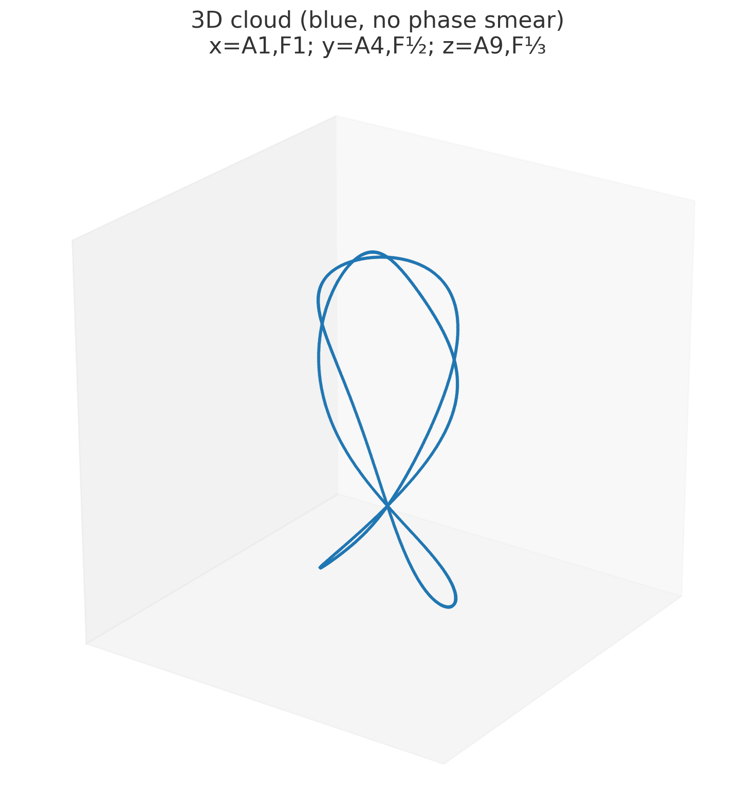
- Calculation of a closed hybrid 9-4-1 oscillation curve 3D hybrid 9-4-1 Orbital, A1F1_A4F½_A9F⅓ cloud (blue)
- Visualization of z-axis indifferent version 3D hybrid 9-4-1 Orbital
What about Schrödinger’s equations?
🌀 Resonant Orbitals as Precession Solutions
In the Olavian Precession Model, each atomic orbital corresponds to a stable resonance between rotational and precessional components of a single oscillating instance — the Roton.
Such a state becomes “quantized” when its motion closes coherently in space and time, forming a self-sustaining geometric figure.
1. Base Assumptions
We describe the motion of a point-like Roton by three oscillatory components
along orthogonal axes:
$$ x(t) = A_1 \sin(\omega_1 t + \phi_1), \quad y(t) = A_2 \sin(\omega_2 t + \phi_2), \quad z(t) = A_0 \cos(\omega_0 t + \phi_0) $$
The parameters $A_i$ define the amplitudes (diameters),
$\omega_i$ the angular velocities, and $\phi_i$ the relative phases.
A configuration is stable when these three oscillations produce a closed 3D trajectory, i.e.
$$ \frac{\omega_i}{\omega_j} = \frac{n_i}{n_j} \in \mathbb{Q} $$
and the geometric figure repeats after a full $2\pi$ rotation.
2. Resonance Condition
For every such stable configuration, the total angular momentum remains constant:
$$ \mathbf{L}(t) = \mathbf{r}(t) \times m\dot{\mathbf{r}}(t) $$
Only specific amplitude–frequency combinations
$(A_0, A_1, A_2, \omega_0, \omega_1, \omega_2)$
produce trajectories where $\mathbf{L}$ precesses harmonically
without drift — these are the resonant orbitals.
The resonance can be stated as:
$$ \Delta \phi = n \pi \quad \text{and} \quad \omega_0 : \omega_1 : \omega_2 = n_0 : n_1 : n_2 $$
yielding a closed-phase manifold equivalent to
the eigenmodes of a standing wave system.
3. Relation to Schrödinger’s Equation
The stationary Schrödinger equation,
$$ \nabla^2 \psi + k^2 \psi = 0, $$
has solutions only for specific $k_n$ values where
the spatial wavefunction fits an integer number of oscillations
into the potential well — a standing-wave condition.
In the precession framework, the same quantization arises when
the rotational and precessional frequencies align such that
the trajectory closes on itself:
$$ \omega_i A_i = \text{const.}, \qquad E_n \propto \sum_i \tfrac{1}{2} m (\omega_i A_i)^2 $$
Thus, the allowed energy levels correspond exactly to
those precession states that meet the resonance-closure condition.
4. Example – The 2p Orbitals
Using the parameter triplets
$$
(A, \omega, \phi) =
([4,1,1], [2,2,2], [0,1,0])
$$
and the three orientations x, y, z:
| Orbital | Orientation | A | ω | φ (× π/2) | Description |
|---|---|---|---|---|---|
| p₂x | x | [4,1,0] | [2,2,2] | [2,0,0] | Linear precession about x-axis |
| p₂y | y | [4,0,1] | [2,2,2] | [0,0,2] | Linear precession about y-axis |
| p₂z | z | [4,1,1] | [2,2,2] | [0,2,0] | Circular (counter-phase) precession producing two lobes along z |
Each corresponds to a harmonic eigenmode of the precession field —
orthogonal, degenerate in energy, and forming the full 2p shell.
5. Interpretation
The Schrödinger orbitals and the Olavian precession figures
describe the same physical principle:
Only those configurations persist whose oscillatory motion
remains phase-locked across all spatial axes.
This recasts quantum eigenstates as geometric resonance figures —
visual, deterministic, and energetically closed in both space and time.
Use the share button below if you liked it.
It makes me smile, when I see it.