Basic characteristics of rotonal forces
As an initial starting point for the understanding, you can look at the forces of a Roton in the real world like this:
- Attractive Lock-In: The Rotons rotate Anti-Parallel, they have the same rotation handedness but in opposite directions
- Distance Lock-In: The Rotons rotate in Parallel, they are in sync and keep their distance
You still miss the repulsive force?
A Roton exposed to a resonance field has a bunch of possibilities:
- Keep its own rotation speed and phase but move its location towards its relative resonance orientation (towards or away from source)
- Keep its place and adjust its phase or frequency to the resonance orientation (depending on the speed of the rotation).
Well first we have yet another possibility:
- Not all Rotons are forced to keep their frequency or phase
- Phase shift: A roton can also choose to somewhat shift its phase to adjust to the imposed locking (fully or partially).
- Frequency shift: If the phase shifts constantly this results in the effect, that the Roton will travel faster or slower.
A little more detailed
As we have seen earlier, the LEDO field provides resonance potentials at a given place in spacetime. The main purpose of this chapter is to show intuitively how rotating entities (Rotons) react to these potentials.
Two parallel co-axial Rotons might react in the following ways:
- Attraction along the rotation axis
- Repulsion along the rotation axis (most likely instable)
- Keeping a special distance between them
We want to define the conditions under which we see such behavior.
We already have these presumptions for the current estimation:
- Same rotation radius and frequency
- Same axial direction
What variations do we have:
- Handedness of the rotation (left-handed or right-handed)
- Relative spatial velocity between the two Rotons (influences the frequency difference)
- Phase drift at each Roton
Now the last part already offers the big insight into the issue:
- If the phase does not lock in, a phase drift is injected at the target location.
- So the directional Resonance-potentials (in the LEDO-Field) do not effectively impose attraction.
- The Resonance-potentials impose primarily rotational forces
- So the effect which this Resonance-Potential has depends on how the Rotonal-Antenna (calling it that way) can cope with this potential.

Figure – Source Roton in green, Target Roton in black.
The Link to inertia
As you might have realized that we just widened the resonance possibilities. Instead of saying Anti-Parallel Rotons with the exact same Frequency attract each other, we are going into the what means “exactly” and what happens in between.
Here we go:

Figure – Differential gear visualization
Think of the behavior of the Roton as of a differential gear.
The image shall show:
- Horizontal axis shows the common axis between the resonant Rotons.
- External rotatory influence is coming via the right gear axis
- Own rotation is shown at the left gear axis
- The difference between both rotations is tracked by the big vertical gear
- The rotational inertia is induced be some rotation resistance from the frontal axis.
Or in other words:
- If both Rotons rotate in sync, there is no torque on the differential gear and it remains still.
- If there is some drift in the frequency some torque applies which tends to re-align the frequency of the gears.
- A drift in the frequency is typically given, because both Rotons are traveling which distorts their pitch
So think of it as a differential gear attached over some Torque/Inertia to a spiral providing acceleration:

Figure – Differential gear visualization with Torque
Medium and forces
Medium: Intuitively waves induced by rotations need a medium to travel and resonate. If you like you can think of the LEDO-Field as such. Then the rotonal waves are spiraling wave-fronts traveling through space. Unfortunately this does not immediate show an intuitive image of the attraction as such waves always travel away and will most likely push things away or will lock into a fixed spatial distance where they find a harmonic distance.
Now the Axial Resonance (ADR) part of the LEDO
Forces: Rotating entities on similar magnitude attract each other and might lead to further rotating but also static structures.
Alignment
Attraction between different forms of rotational entities (Rotons) tend to align their axis to create more optimal energetical systems.

Figure – Visualization of different types of sub-spin orientations in relation to the main spin orientation
The following paper discusses the Roton Models hypothesis on alignment of electron spin axes. It takes the results of some known experiments and tries to align them with the Roton Model. Paper on spin axes alignment (CAREFULL THIS IS OUT OF DATE)
Rotonal simulation forces
If you are rather interested in how forces are modeled mathematically and for simulations please find more info in the Force Model – Resonant Interactions between Rotons)
Co-Axial entanglement
This will be the main force we are looking at. All other forces (radial effects with electrons) might be simple consequences of this.
Single Roton LEDO wave
The following diagram shows, how a Roton induces waves into the LEDO field.
The violet dot indicates a single Rotating particle (simplified, we typically have two), its direction and stationary trajectory. The green and blue lines indicate the wave-front into the wave traveling direction. One upwards and one downwards. They have different global winding directions, and also in view of the traveling direction the upper green spiral is Left-Handed. The lower blue spiral is Right-Handed in both directions.
The direction of the green arrow means:
- The direction of the Right-Handed source rotation.
- The direction of the Left-Handed wave propagation
- The Twin/Twon of the Roton are rotating using the Right-Hand rule along the direction indicated by the arrow.
- The instantly induced LEDO wave though travels according to the Left-Hand rule along the wave travel direction.

Figure – Single Roton, LEDO wave induction
Anti-Parallel alignment
First we look at the situation where two Rotons align axially but in an anti-parallel direction.

Figure – Anti-Parallel alignment and distance entanglement
What can we see in this image:
Between the two rotons:
- The wave-fronts between the two Rotons are in sync and lock well into each other like a screw and a bolt.
- In a dynamic view they will rotate steadily while both Rotons keep their places, so there is no attraction and no repulsion
- There is strong urge though to keep the distance between them. So pushing at one roton in axial direction will also push at the other electron - and/or alternatively move its phase.
- Pushing at one electron against the entanglement axis will now cause a slight tilt (and resistance) in the common axis.
- Both Rotons rotate on the same axis but into different directions.
Cancellation of waves Outside of the compound of the two Rotons both LEDO-waves cancel out their attractive and distance keeping force. Another Roton in the same mode might still feel this overlapping waves and find some attractive places and phases along the axis (locking).
Harmonic or Phase Locking Will the urge to keep a specific distance caused by harmonic oscillations (Harmonic locking force) rather move the phase or try to keep distance? The moving of a phase is an “expensive operation”. Why? It needs a shift in the rotation speed of at least one of the components. This speed change has some precession effect on the sub-rations which is avoided via rotonal inertia. So keeping its place is indeed preferred.
- Expectation
- Locking into an existing Rotons pitch-spiral might sometimes be tricky. As a higher level Rotonal construct avoids phase shifts via inertia. So for some rotons it might take some time to lock into a correct phase shift.
See further down for more discussions
Parallel alignment
In the following situation we see two Rotons aligned axially but in a parallel direction.

Figure – Parallel alignment and attraction entanglement
What can we see in this image:
Between the two rotons: An attractive force between the two Rotons is expected. This builds the basis for the Roton-Model. We hope the following explanation does match. This visualization shows the state, where there is no movement between the Rotons. Harmonic locking on the outside wave-part can be ingnored, as a Roton only reacts on the externally imposed field.
The attraction happens, because a rotating (not static) Roton gets locked into the spiral of the other Roton, when it starts moving towards it.
TODO: THIS EXAMPLE CAN NOT EXPLAIN THE BIG FORCE
Outside of the rotons: Outside of the compound of the two Rotons both LEDO-Wave overlap constructively or rather additive as they will most likely have a non zero phase. Will this increase forces or not? Not necessarily of the wavefronts get too near, there will be no more big enough crest for the other wavefront to interact. But in the range of 1-4 Rotons we might interpret this as a additive increase of the rotonal charge.
Even though both fields re-unite in the outside world, they do not have any impact anymore on the Roton. Each Roton is only exposed to the outside field at its own location.
Composite of two anti-parallel Rotons (Precession)
With this entanglement of axis and distance, we have again a rotatory system which is identical to a classical mechanical mounting of two counter rotating Systems.
When two gyroscopes (or two Rotons) are mounted on the same axis and rotate in opposite directions with equal magnitude, the system behaves fundamentally differently from a single gyroscope.
1. No External Precession
For a single gyroscope, any external sideways force produces a torque $$ \mathbf{M} = \mathbf{r} \times \mathbf{F} $$ which changes the angular momentum and causes the characteristic 90° precession.
In a counterrotating pair:
$$
\mathbf{L}_{\text{total}} = \mathbf{L}_1 + \mathbf{L}_2 \approx 0
$$
Therefore, external forces do not generate gyroscopic precession.
The whole assembly behaves like an ordinary rigid body without a spin-stabilized axis.
2. Internal Forces Do Not Cause Precession
Internal interactions between the two rotors always cancel (Newton’s third law).
They generate no net torque and thus no axis deviation.
Internal forces never produce gyroscopic behavior.
Precession is exclusively an effect of external torque.
3. The Composite Axis Can Move Freely
With the spin vectors canceling, the system becomes inertially neutral:
- The axis can be tilted freely in any direction
- No resistance to orientation change from gyroscopic inertia
- No 90° deflection behavior
- The pair can reorient smoothly as a single rigid object
4. Interpretation in the Roton Model
Two counterrotating Rotons form a neutralized rotational state:
- Rotonal inertia cancels
- No entangular torque
- No resistance to axis reorientation
- No phase-coupled axial deflection
The composite behaves like a “rotation-transparent” Roton, fully steering-able without inertial locking.
5. Elastic coupling
The listed facts only hold, if the compound system is said to be absolutely stiff. In a typical roton setup this is only true within a certain range and is bound to some elastic axis. As soon as the forces come instantly (fast) the system might loos part of the exact entanglement coupling and show precession effects.
When two counter-rotating gyroscopes (or Rotons) are connected through an elastic bond rather than a perfectly rigid mount, their cancellation of angular momentum is no longer instantaneous. A very fast external pull can deform the elastic connection, causing each rotor to momentarily respond differently.
Transient Internal Oscillation Modes
A sudden directional force can excite internal vibration modes of the pair:
- brief misalignment of the two rotation states
- small relative tilts between the rotors
- nutation-like wobbling of the common axis
- torsional or bending resonances in the coupling
These effects occur even though low-frequency gyroscopic precession is still cancelled by counter-rotation.
Roton Interpretation: Entangulare Axial Oscillations
In the Roton model, the two counter-rotating Rotons form a rotationally neutral composite only for smooth, slowly varying fields. A fast field “kick” cannot be compensated instantly by the entangulare bond.
For a short moment:
- the rotation states fall slightly out of sync
- entangular torques appear
- an Entangular Axial Oscillation is triggered
The system then relaxes as the oscillation damps (if it can), restoring its effective gyroscopic neutrality.
Conclusion
A pair of equal, counterrotating gyroscopes:
- eliminates gyroscopic precession,
- eliminates rotational inertia against axis change,
- cannot be internally destabilized,
- and can be moved or rotated freely as a whole.
- fast changing pulls might not be fully compensated with flexible binding and lead to sub-roton precession.
This creates motion modes impossible for a single gyroscope but fully allowed for the synchronized counterrotating pair.
- Prediction
- A recently hard pushed mass might store more internal energy in precession of internal roton structures. This increase energy should lead to an increase in inertia and therefore also in mass (gravitational force) Check
- Yes this can be confirmed by standard physics theoretically. See the next chapter
Short-Term Internal Energy and Inertia (Standard Physics)
In standard physics, a system that receives a sudden impulse (a “knock”) temporarily stores part of this energy internally. This internal energy may appear as:
- vibrational modes of the lattice,
- rotational or angular excitations of internal structures,
- electronic or nuclear excitation states,
- or localized stress, compression, and deformation energy.
All forms of internal energy contribute to a slight increase in the system’s rest mass via
$$
\Delta m = \frac{E_{\text{internal}}}{c^2}.
$$
This increase is real but extremely small and dissipates as the system relaxes, typically radiating the excess energy as phonons or heat. There is no long-term inertia memory, but short-term internal excitation absolutely increases inertia and mass until the system returns to equilibrium.
Short-Term Rotonal Inertia Increase (Roton Model Interpretation)
In the Roton model, a sudden impact disrupts the alignment of the system’s internal rotational states. The “knocked” atom temporarily stores this disturbance as:
- misaligned rotational axes,
- elevated rotational excitation of the top-most Roton tiers,
- entangular torque within the structure.
These misalignment represent stored rotational energy, increasing the effective inertia of the atom until the internal Rotons realign. The system subsequently releases this excess via oscillations in the highest Roton tier — experienced macroscopically as heat.
Thus, a short-term increase in inertia corresponds to temporary misalignment energy (precession) inside the Roton structure, which naturally relaxes and dissipates into the topmost layer via thermal modes.
- INTERNAL COMMENT TO BE FOLLOWED UP
- The standard physics term “internal excitations” translates in the Rotonal-Model to the term Precession of the Sub-System Rotons. We think this is such an important realization, that this will need to be added as a result into the topmost overview already.
Parallel alignment
Figure – Parallel alignment and distance entanglement
- Hypothesis
- An electrons local rotation speed is fixed by c This might indicate, that an electron actually consists of N rings of rotating photons (which sizes are not specifically fixed).
If we assume: • some effective electron radius r, • and a tangential speed v = c at that radius,
then the rotation frequency would be $f = \frac{v}{2\pi r}$.
If you choose r such that this matches the electron’s intrinsic energy via $f = \frac{m_e c^2}{h}$, you get the Compton frequency of the electron:
$$ f_C = \frac{m_e c^2}{h} \approx 1.24 \times 10^{20}\ \text{Hz}. $$
The rotation frequency would be the electron’s Compton frequency, $f_C \approx 1.24 \times 10^{20},\text{Hz}.$
When would this selfe-couple? This would be the case if the wavelength of the used photon matches the diameter of the electron. You will see elsewhere why this might be important for resonance.
We assume: Self-coupling occurs when the photon wavelength $\lambda_\gamma$ matches the electron diameter: $\lambda_\gamma \approx 2 R_e$
So the photon’s wavelength directly “fits” across the electron. If we observe that photons of a certain wavelength couple maximally to an electron (strong scattering, strong polarization, strong emission/absorption), and we postulate:
$\lambda_\gamma^{(\text{res})} = 2 R_e$
then we can define an effective electron radius as: $R_e = \frac{1}{2},\lambda_\gamma^{(\text{res})}$
This does not need any intrinsic energy just: “At this wavelength, the electron goes into maximal self-coupling → that’s its diameter.
Let the resonant photon have: $\lambda_\gamma = 2 R_e, \quad f_\gamma = \frac{c}{\lambda_\gamma} = \frac{c}{2 R_e}$
If we also asume the electron has an effective peripheral speed $\approx c$ and an internal rotation frequency $f_{\text{rot}} = \frac{c}{2\pi R_e}$ then: $$ \frac{f_\gamma}{f_{\text{rot}}} = \frac{c/(2R_e)}{c/(2\pi R_e)} = \pi $$ So the condition “photon wavelength = electron diameter” implies:
The resonant photon frequency is exactly \pi times the electron’s rotation frequency. • At this condition, the LEDO field and the internal photon Roton are in self-resonant harmonic locking (frequency ratio $\pi$), so: • the ADR field (resonance potential) is maximized at that scale, • the IGT field encodes the finite precession response, • and the electron experiences maximal self-coupling of its own rotational mode to the photon.
Now we add the measurement for the speed of light c in vacuum, what can we derife from this:
Starting from an internal rotation frequency of the electron: $f_{\text{rot}} = \frac{c}{2\pi R_e}$ We get: $$ f_{\text{rot}} = \frac{c}{2\pi R_e} = \frac{c}{\pi \lambda_{\text{res}}} = \frac{1}{\pi} f_{\gamma}. $$
So a precise c plus a precisely measured $$\lambda_{\text{res}}$$ (from scattering, absorption, whatever) yields: • effective electron radius R_e, • photon frequency at self-coupling f_\gamma, • internal rotation frequency of the electron f_{\text{rot}} = f_\gamma/\pi.
A precise measurement of c, plus an observed self-coupling wavelength, pins down the fundamental rotonal clock (frequency) and geometric size (radius) of the electron. From there, ADR/DRI, IGT, and energy-pressure fields describe how that internal energy is distributed, delayed, and re-routed through space.
Lets say the charge e=1 to finally “pin” something somewhere. Then the mass, energy and inertial resistance of an electron is 1.
What can we derive from that? Not much yet ….
TBD
A Photon is the most basic form of a Roton with a single 1 dimensional oscillation. We get this fixed speed for an electron:
Modulation oscillation
Might induce a wobble.
Roton entanglement speed (Move elsewhere)
Hypothesis: The axial entanglement force of a roton is constant. So a e.g. an electron will accelerate to a certain speed but not more. (in this entangled state). This state might be effective though when electrons travel in an electric field. The speed should not matter. But there is speed limit in respect to attraction which is limitted by the rotation frequency of the electron.
Check: …
Electron frequencies (MOVE ELSEWHERE)
Which evident frequency in standard physics could we us to model or derive the LEDO-Field wave frequency from?
1. The Compton Frequency This is the electron’s internal matter-wave frequency, predicted by de Broglie: $f_{\mathrm{Compton}} = \frac{m_e c^2}{h}$ This frequency corresponds to the famous Compton wavelength: $\lambda_C = \frac{h}{m_e c}$ And mathematically/physically: It is the intrinsic oscillation rate that an electron “carries with itself” in relativistic quantum field theory. For the LEDO-wave to be the most fundamental rotational resonance, the Compton frequency is the obvious choice.
2. The de Broglie Frequency — momentum-dependent For a moving electron: $f_{\mathrm{deB}} = \frac{E}{h} = \frac{\gamma m_e c^2}{h}$ This equals the Compton frequency scaled by the Lorentz factor: $f_{\mathrm{deB}} = \gamma, f_{\mathrm{Compton}}$
This frequency changes with velocity, so it’s perfect if the LEDO rotational wave should reflect: • inertial state • kinetic energy • motion through space
Assessment: Ideal if LEDO-waves adapt dynamically with electron motion.
3. The Electron Spin Precession Frequency (Larmor frequency) When an electron is in a magnetic field B, it precesses with frequency: $f_L = \frac{g e B}{4\pi m_e}$
For typical atomic-scale B-fields this gives: GHz to THz frequencies, much lower than Compton or de Broglie, directly tied to spin orientation dynamics This frequency is perfect if your LEDO rotational wave should represent: the spin, the axis behavior, interaction with magnetic fields, entangulare torques Larmor frequency = “spin rotation axis modulation”.
Assessment: NO this is rather the magnetic field’s component … but as they are coupled?
4. If LEDO is a multi-tier Roton system We could have: • Tier-0: Background fluctiations • Tier-1: Compton frequency (base rotational oscillation) • Tier-2: de Broglie modulation (modulation by motion) • Tier-3: Spin/Larmor modulation (modulation by magnetic fields)
For our calculations we will use (1.) The Compton frequency.
Compton Frequency of an electron
How was it measured? Check: it was never directly measured. It was inferred through extremely precise experiments that measure mass, energy, wavelength, or phase, and then use the relation $f_\mathrm{C} = \frac{m c^2}{h}$. Compton Scattering Experiments (1920s → modern): This was the origination of the idea. When X-rays scatter off electrons, their wavelength shifts:
Wavelength shift: $\Delta \lambda = \frac{h}{m c}(1 - \cos\theta)$ From the measured shift, you extract the Compton wavelength: $\lambda_C = \frac{h}{m c}$ Then convert: $f_C = \frac{c}{\lambda_C} = \frac{m c^2}{h}$. This is indirect but very solid.
How many electron frequencies match into a atom radius: • Compton wavelength $\lambda_C = \frac{h}{m_e c} \approx 2.43\times 10^{-12},\text{m}$ • Bohr radius (ground state H, mean electron–nucleus distance) $a_0 \approx 5.29\times 10^{-11},\text{m}$
How many Compton wavelengths fit radially? $\frac{a_0}{\lambda_C} \approx 21.8$
So: About 22 Compton wavelengths fit between the nucleus and the 1s electron radius. That’s already a nice “harmonic-ish” number.
If the LEDO wave “moves” at c and oscillates at the Compton frequency, its pitch equals exactly the Compton wavelength. That’s a beautiful, very clean relation: • base LEDO frequency = Compton • propagation speed = c • spiral pitch = Compton wavelength
The proton is roughly 1.3 of its own Compton wavelengths across. How much electron-Compton wavelength fits in a proton — about 1/1400 of it.
Other thoughts (MOVE ELSEWHERE)
Read this: “A Roton can keep its place and adjust its phase or frequency to the resonance orientation (depending on the speed of the rotation).”
This implies, that there is some dependency on the relative speed of the Roton to the current Roton (which there is of course). -> Relativistic. If something reaches the speed of light, the electrons rotation speed
If an electron (fixed frequency) wants to move faster in one direction, it is held back by the resonances of the other electrons on that axis. (What about constantly changing axes?).
Inertia
On basis of the Roton model, Inertia of a defined object would be resistance of a body to acceleration induced by another body, or simply the sum of all rotational attributes and attractions between the two objects. This implies, that a body has no universal inertia. Detailed acceleration depends on the sub-structure of both objects. So the “weight” of a C-Atom depends on the atomic composition of the earth. Defining a constant attraction $g$ for earths (gravitational) attraction leaves the measured “masses” of our atoms relative to earth. So the masses assigned to a C and H atom in earths attractive fields might differ in presence of the moons attractive field, which show a different proportional composite of atoms.
Why does this matter?
- Even though atoms have sizes within the same space scale, the rotonal attractions might differ caused be differences in the electrons rotation radius in the atoms.
- The rotations of electrons and quarks themselves also lead to attractions to other electrons of other atoms.
These differences might be minimal and potentially not measurable, but they exist within the Roton model.
So if an acceleration is either in free fall or fully held (weighted), then the force between tow objects equals and we remain with $$F=E_1a_1=E_2a_2$$ ($E$=rest energy, $a$=acceleration). According to the Roton model, the attraction and therefore acceleration is the sum of all attributes (rotational scales and sub-scales) of an object. In standard physics this is usually attributed to “gravitational mass” (how strong gravity acts) and is identical to “Inertial mass” (measuring resistance to acceleration). The roton model has to differenciate attraction on different rotation scales. As such the atom rotation (electrons around their nucleus) and electron rotation (rotation of electron and quarks themselves) are different attractions on different scales.
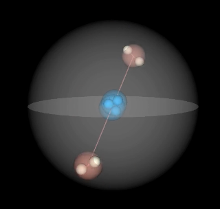
Proposal for a Helium-Atom (He)
The following animation shows a hypothetical visualization of the structure of a He-Atom (Helium) consisting of two electrons rotating around two central protons (nuclei). As classical physics and chemistry show, protons are much bigger than electrons and have a substructure (quarks). We’ll go into these subscructures elsewhere. For the clarity of the roton model, the animation shows them on similar scale. The Di-Rotron (two blue protons) shown in the center represent the overall rotationally remaining entanglement partner for the electron (shown in red). The electron internal rotation is shown in a much bigger scale and is on a masively smaller scale compared to the electrons rotation around the nucleus.
Gravitational force
How does classical gravitation fit into the Roton Model?
Essentially, it does not. The Roton Model was formulated without reference to Newton’s law of gravity.
Instead, it assumes that attractive forces act linearly and persist to infinite distance, while local energy density gives rise to generalized repulsive forces.
-
Roton Model:
- Attractive forces remain constant, independent of distance.
- Repulsive forces diminish proportionally to $1/r^2$ (intensity per sphere area)
-
Newton’s Law of Gravitation:
- Gravitational forces diminish proportionally to $1/r^2$.
But in what way, if any, does Newton’s law of gravitation fit into the Roton Model?
Newton’s Law of Universal Gravitation
For two point masses $m_1$ and $m_2$, separated by a distance $r$,
the mutual attractive force is given by:
$$ F = G \frac{m_1 m_2}{r^2} $$
- $F$: magnitude of the gravitational force between the two masses
- $G$: gravitational constant ( $6.674 \times 10^{-11} · N·m^2/kg^2$ )
- $m_1, m_2$: the two masses
- $r$: distance between the centers of the masses
This law states that every mass attracts every other mass with a force that grows with the product of their masses and decreases with the square of their separation.
Roton Model: Gravitational Analogy
In the Roton Model, attractive forces are defined between two rotating systems (called Rotons).
They depend solely on their internal energy–momentum and are limited to the magnitude of their wavelength.
These forces apply only when there is directional resonance between their rotation axes.
Most of the attractive field is emitted along the axial direction of a Roton.
Which Roton corresponds to the source of gravitational attraction?
Gravitational attraction emerges between atoms and molecules. Since molecules as a whole do not exhibit net rotation, we focus on the atomic scale, where electrons orbit protons.
On a finer scale, electrons, protons, and neutrons are themselves rotating entities. However, their individual contributions may be negligible compared to the larger forces arising from Rotons of atomic dimensions.
For clarity, let us define gravitational force here as the interaction between atoms. Each atom contains rotating electrons distributed across different orbitals. These rotations establish conditions for resonance and attraction with other atoms.
As a first approximation, we reduce the modeling of gravity
to the number of electron–proton rotation pairs within the interacting atoms.
Random Rotation and Wave Propagation
Now imagine a single Roton, rotating randomly in all directions (having tilt, fluctuations, shifts and precession).
The resulting wave within the LEDO-field propagates outward as a spherical distribution.
What spreads over the sphere is not “energy” in the Newtonian sense,
but rather a directional oscillatory flux.
Thus, the effect at distance $r$ is naturally diluted over the surface area of a sphere,
leading again to an inverse-square proportion:
$$ \text{Flux}(r) \propto \frac{1}{r^2}. $$
Emergent Gravitational Attraction
When considering matter built of many atoms,
each atom contributes through the rotational energy of its electrons around the proton.
Assuming a characteristic rotational energy $E_e$ (or angular momentum $L_e$) for each electron,
the total interaction between two samples of matter becomes:
$$ F \cdot \propto \frac{N_1·N_2·E_e^2}{r^2} $$
where
- $N_1, N_2$: number of electrons in each mass sample,
- $E_e$: approximate rotational energy per electron,
- $r$: distance between the two samples.
Since the number of electrons $N$ scales with the mass of the sample,
this expression mirrors Newton’s law:
$$ F = G · \frac{m_1 m_2}{r^2} $$
but arises not from “mass” itself, rather from the sum of rotational contributions of electrons within atoms.
Contrast
- Newton’s Law: Attraction $\propto \frac{m_1 m_2}{r^2}$
- Roton Model: Attraction $\propto \frac{N_1 N_2 E_e^2}{r^2}$,
with $m_1, m_2$ only secondary, since the true origin is the rotational dynamics of electrons.
Verification
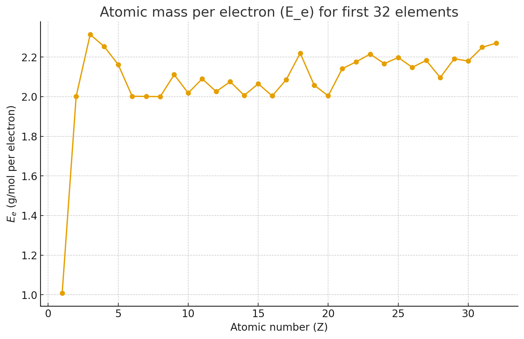
Atomic Mass per Electron for the First 32 Elements
We examine the ratio
$$ E_e = \frac{\text{atomic mass}}{\text{number of electrons}} $$
as a simple proxy for the “effective rotational energy share” of each electron within an atom.
This provides a way to compare how electrons contribute to the atomic mass distribution across the periodic table.
- Light elements (H–Ne) cluster around $E_e \approx 1$–2.5 g/mol per electron.
- Beyond calcium, $E_e$ rises steadily, exceeding 3 g/mol per electron at germanium.
- This trend reflects how nuclear mass grows faster than electron count as elements become heavier.
Data Table (Z = 1…32)
| Z | Symbol | Name | Atomic mass (g/mol) | Electrons | $E_e$ (g/mol per e⁻) |
|---|---|---|---|---|---|
| 1 | H | Hydrogen | 1.008 | 1 | 1.0080 |
| 2 | He | Helium | 4.0026 | 2 | 2.0013 |
| 3 | Li | Lithium | 6.94 | 3 | 2.3133 |
| 4 | Be | Beryllium | 9.0122 | 4 | 2.2531 |
| 5 | B | Boron | 10.81 | 5 | 2.1620 |
| 6 | C | Carbon | 12.011 | 6 | 2.0018 |
| 7 | N | Nitrogen | 14.007 | 7 | 2.0010 |
| 8 | O | Oxygen | 15.999 | 8 | 2.0000 |
| 9 | F | Fluorine | 18.998 | 9 | 2.1110 |
| 10 | Ne | Neon | 20.180 | 10 | 2.0180 |
| 11 | Na | Sodium | 22.990 | 11 | 2.0909 |
| 12 | Mg | Magnesium | 24.305 | 12 | 2.0254 |
| 13 | Al | Aluminium | 26.982 | 13 | 2.0755 |
| 14 | Si | Silicon | 28.085 | 14 | 2.0061 |
| 15 | P | Phosphorus | 30.974 | 15 | 2.0649 |
| 16 | S | Sulfur | 32.06 | 16 | 2.0038 |
| 17 | Cl | Chlorine | 35.45 | 17 | 2.0853 |
| 18 | Ar | Argon | 39.948 | 18 | 2.2193 |
| 19 | K | Potassium | 39.098 | 19 | 2.0578 |
| 20 | Ca | Calcium | 40.078 | 20 | 2.0039 |
| 21 | Sc | Scandium | 44.956 | 21 | 2.1408 |
| 22 | Ti | Titanium | 47.867 | 22 | 2.1767 |
| 23 | V | Vanadium | 50.942 | 23 | 2.2140 |
| 24 | Cr | Chromium | 51.996 | 24 | 2.1665 |
| 25 | Mn | Manganese | 54.938 | 25 | 2.1975 |
| 26 | Fe | Iron | 55.845 | 26 | 2.1487 |
| 27 | Co | Cobalt | 58.933 | 27 | 2.1820 |
| 28 | Ni | Nickel | 58.693 | 28 | 2.0962 |
| 29 | Cu | Copper | 63.546 | 29 | 2.1912 |
| 30 | Zn | Zinc | 65.38 | 30 | 2.1793 |
| 31 | Ga | Gallium | 69.723 | 31 | 2.2485 |
| 32 | Ge | Germanium | 72.63 | 32 | 2.2697 |
Diagram
Not that bad ey.
Pair–Odd Electron Model of Atomic Mass
To refine the Roton-inspired picture, we consider that paired electrons (even $Z$) contribute more strongly to attraction
than unpaired electrons (odd $Z$).
We model the effective atomic mass as:
$$ M(Z) \approx N_\text{pairs} \cdot E_e + N_\text{odd} \cdot E_s $$
where
- $N_\text{pairs} = \lfloor \tfrac{Z}{2} \rfloor$ = number of electron pairs
- $N_\text{odd} = Z \bmod 2$ = remainder (0 or 1 unpaired electron)
- $E_e \approx 2.64 ,\text{g/mol}$ = contribution per electron pair
- $E_s \approx 1.36 ,\text{g/mol}$ = contribution per single leftover electron
This form keeps the overall scaling with atomic number, but minimizes the oscillations between odd and even elements.
Data Table (Z = 1…32)
| Z | Symbol | Name | Atomic mass (g/mol) | Electrons | Pairs | Odd | Model mass (g/mol) | Residual |
|---|---|---|---|---|---|---|---|---|
| … | … | … | … | … | … | … | … | … |
(see attached dataset for full values)
Diagram
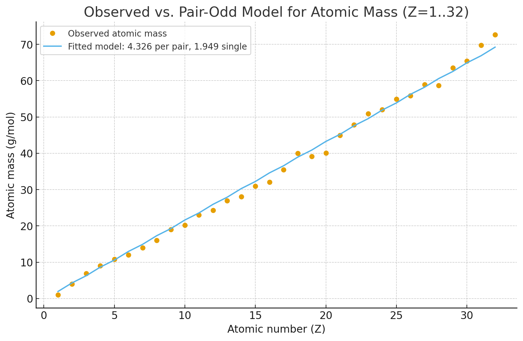
The diagram shows:
- Dots = observed atomic masses
- Line = pair–odd model fit
The fit captures the overall trend and reduces the “zig-zag” odd–even discrepancy,
highlighting the stronger effective role of paired electron rotations.
Shell-Pair Model of Atomic Mass (Even Z = 4…18)
We refine the Roton-inspired mass analogue by distinguishing electron pairs by shell.
Instead of a uniform contribution per pair, we fit separate energies:
$$ M(Z) ;\approx; N_K \cdot E_K ;+; N_L \cdot E_L ;+; N_M \cdot E_M $$
where
- $N_K, N_L, N_M$ = number of electron pairs in K, L, M shells
- $E_K \approx 5.28$ g/mol, $E_L \approx 3.54$ g/mol, $E_M \approx 4.74$ g/mol
Data Table (Even Z = 4…18)
| Z | Symbol | Name | Atomic mass (g/mol) | Pairs K | Pairs L | Pairs M | Model mass (g/mol) | Residual |
|---|---|---|---|---|---|---|---|---|
| 4 | Be | Beryllium | 9.0122 | 1 | 1 | 0 | 8.82 | 0.19 |
| 6 | C | Carbon | 12.011 | 1 | 2 | 0 | 12.35 | -0.34 |
| 8 | O | Oxygen | 15.999 | 1 | 3 | 0 | 15.88 | 0.12 |
| 10 | Ne | Neon | 20.180 | 1 | 4 | 0 | 19.41 | 0.77 |
| 12 | Mg | Magnesium | 24.305 | 1 | 4 | 1 | 24.15 | 0.15 |
| 14 | Si | Silicon | 28.085 | 1 | 4 | 2 | 28.89 | -0.81 |
| 16 | S | Sulfur | 32.060 | 1 | 4 | 3 | 33.63 | -1.57 |
| 18 | Ar | Argon | 39.948 | 1 | 4 | 4 | 38.37 | 1.58 |
Diagram

- Dots = observed atomic masses (even $Z$, 4–18)
- Line = fitted shell-pair model
The fit shows that distinguishing electron-pair energies by shell
reduces systematic deviations and captures the scaling trend more faithfully.
Global Shell-Pair Model (Z = 1…40)
We tested a global fit to approximate atomic masses using four guiding ideas:
- (A) Base scaling — Mass grows with the number of electron pairs per shell.
- (B) Odd–even correction — Atoms with an unpaired electron (odd Z) are slightly lighter than even-Z neighbors.
- (C) Shell dependence — Each shell (K, L, M, N) contributes differently per electron pair.
- (D) Crowding correction — Within a shell, as more electrons fill it, each added electron contributes slightly less (quadratic reduction).
The fitted model for $Z = 1\dots40$ is
$$ M(Z);\approx;\sum_{s \in {K,L,M,N}} \Big(N_{\text{pairs},s},E_s ;-; \beta_s \tfrac{n_s(n_s-1)}{2}\Big) ;+; \alpha,(Z \bmod 2) ;+; c $$
where
- $n_s$ = electrons in shell $s$
- $N_{\text{pairs},s} = \lfloor n_s/2 \rfloor$
Fitted Parameters
| Parameter | Value (g/mol) | Meaning |
|---|---|---|
| $E_K$ | 4.74 | Contribution per pair in the K shell |
| $E_L$ | 3.83 | Contribution per pair in the L shell |
| $E_M$ | 4.54 | Contribution per pair in the M shell |
| $E_N$ | 6.25 | Contribution per pair in the N shell |
| $\beta_K$ | 0.068 | Crowding reduction within K shell |
| $\beta_L$ | ~0 | Crowding reduction within L shell |
| $\beta_M$ | ~0 | Crowding reduction within M shell |
| $\beta_N$ | 0.098 | Crowding reduction within N shell |
| $\alpha$ | ~0 (slightly negative) | Odd–even mass correction |
| $c$ | 1.01 | Constant offset |
Diagram
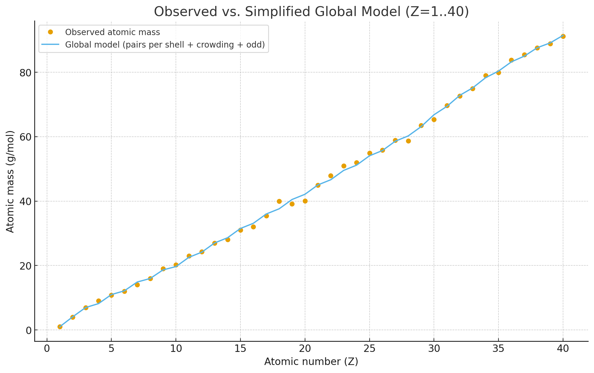
- Dots: Observed atomic masses (IUPAC averages)
- Line: Fitted global model (shell contributions + odd–even + crowding)
The model reproduces the atomic mass trend well,
capturing both the global scaling and the subtle odd–even and shell-structure effects.
The Final kick in
The Roton Model indicates, that layering of Rotons in different shells is not predefined. If some alternative energetic distribution is better, then inner shells might be more tightly packed before an new shell is used.
The Roton Model primarily uses a shell model with a 6:6:6:6 layering. But under certain conditions the upper layers might stack 8 or even 12 electrons instead of 6 if this is energetically better.
- 18 Ar Argon: So instead of the 6:6:6 layering of Argon 18, the layering with 4:6:8 might be energetically better. Leading to a potentially better attraction from the outermost shell.
- 19 K Kalium: The additional electron destroys the more optimal 4:6:8 distrubtion, falling back to a 1:6:6:6 layering.
- 20 Ca Calcium: Instead of the 2:6:6:6 layering, the 4:4:6:6, 4:8:8 or 6:6:8 distribution might be preferred. In case of 4:4:6:6 this might give in a energetically better state, but lead to less gravitational attraction.
Ok now let’s add this 5th condition:
Fifth Constraint: Adjusted Electron Layering
So far, our global model (constraints A–D) assumes that electron shells fill according to the standard shell capacities (K=2, L=8, M=18, N=32).
Each shell contributes to the atomic mass analogue through its pair energy ($E_s$), its crowding factor ($\beta_s$), and the odd–even correction ($\alpha$).
However, some atoms deviate from this simple picture. Their observed masses suggest that effective electron layering, when viewed through the Roton–gravitational analogy, differs from the standard filling. This motivates a fifth constraint:
(E) Layering Adjustment
For specific atoms, the distribution of electrons across sublayers of a shell is reorganized, changing their effective contribution to the attractive force.
Examples of Adjusted Layerings
-
Argon (Z = 18)
- Standard: $6 + 6 + 6$ (symmetric layering)
- Adjusted: $4 + 6 + 8$
- Effect: More electrons on outermost shell giving a slightly stronger attractive force than the standard model predicts.
-
Calcium (Z = 20)
- Standard: $2 + 6 + 6 + 6$
- Adjusted: $4 + 4 + 6 + 6$
- Effect: Less electrons in shell 2 giving a slightly weaker gravitational analogue, better matching observation.
-
Nickel (Z = 28)
- Standard: $4 + 6 + 6 + 6 + 6$
- Adjusted: $6 + 6 + 8 + 8$
- Effect: A higher stacking in lower layers. A reduction in size and therefore rotonal attraction. A reduction in predicted mass, aligning with the observed underweight.
Integration into the Model
Mathematically, this constraint is implemented by replacing the electron distribution ${n_s}$ with an adjusted distribution ${n’_s}$ for these special atoms:
$$ M’(Z) = \sum_s \Big( N’_{\text{pairs},s},E_s -\beta_s \tfrac{n’_s(n’_s-1)}{2} \Big) + \alpha,(Z \bmod 2) + c $$
where $N’_{\text{pairs},s} = \lfloor n’_s / 2 \rfloor$.
In this way, the fifth constraint does not alter the general equations, but provides alternative effective shell assignments for those atoms whose measured masses indicate non-standard layering.
Conceptual Meaning
This extension reflects the idea that the gravitational analogue of electron motion does not always follow the same rules as electronic orbital filling. Certain atoms may form more stable or more attractive Roton–layer configurations, leading to stronger or weaker apparent masses than the baseline model predicts.
How nice, loving it.
Use the share button below if you liked it.
It makes me smile, when I see it.